An introduction to the Laplace Transform

This is a generalisation of the more common Fourier transform, which is known for image compression because it can decrease computation time.

The Laplace transform is defined by

where  is the complex Laplace variable and  is the function you want to transform.

Don’t worry if you have never seen this before: this part is often done with a computer anyway. In essence though, the transform “translates” the function of  into a function of the Laplace variable, .

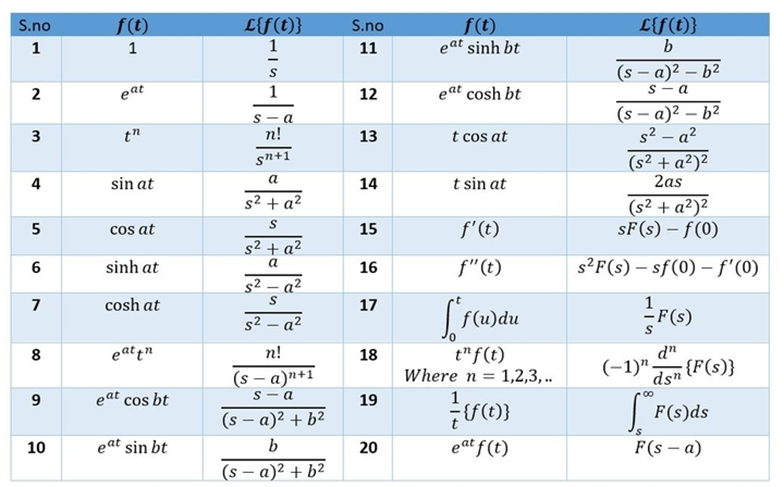
The important thing is that the Laplace transform is a linear operator. This means that if you had another linear operator, say a multiplication by three, you would be able to use the operators in either order to get the same answer. It is our luck that derivatives act as linear operators too. This leads to some interesting properties, as summarised by S.no 15 and 16 (all of these are important in practice)

Figure 1 - (BYJU's Exam Prep, 2023)

As such, whatever differential equation you have, you can transform it and factorise out  to get the Laplace transform of your function. It is advisable to define the boundary conditions at this point. Now comes the hard part: the inverse-Laplace transform. This is defined by

where S=Y  is any complex line to the right of all the poles of. The integral can be done by hand or the table can be used, but generally this part is best left for computers. As such, we now have a function of  which, to obtain, we would have otherwise needed to use iteration.

Example 1: spring oscillator

Let us say we want to derive the equation for a mass oscillating on a spring as a result of a perturbation. The following equation holds true:

where  is x is displacement as a function of time. This will be our respective f(t) , but we will call it x(t) to minimise confusion. Laplace transform both sides to get

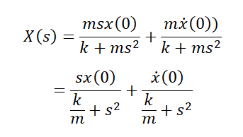
Rearrange this for X(s) to get

This already somewhat looks like the S.no 4 and 5 entries in the table, but the key is to remember that addition, multiplication and the reverse-Laplace transform are linear functions, so one can split up the above fraction into smaller fractions. Then, each part can be reverse-Laplace transformed individually and added to get a total answer. The first step is to rewrite the terms in a compatible form (i.e. find the values of  from the table in S.no 4 and 5).

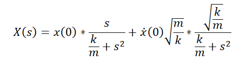
Now it is obvious that a^2  is k/m, the above can be written as

and this can be reverse-Laplace transformed to

This is indeed . the general solution for simple harmonic motion, where x (0)  is the initial velocity of the spring,  is the spring constant,  is the mass of the oscillating mass and x(0) is the initial position.

Example 2: spring oscillator with drag/damping

Now imagine a spring moving through a viscous liquid: the spring will eventually stop oscillating, its amplitude dying out. This kind of motion is called damped harmonic oscillation. We can model this with

where c is a positive constant used to control the level of damping in the system. It is recommended you start work through the problem as you read along. Laplace-transform both sides as before.

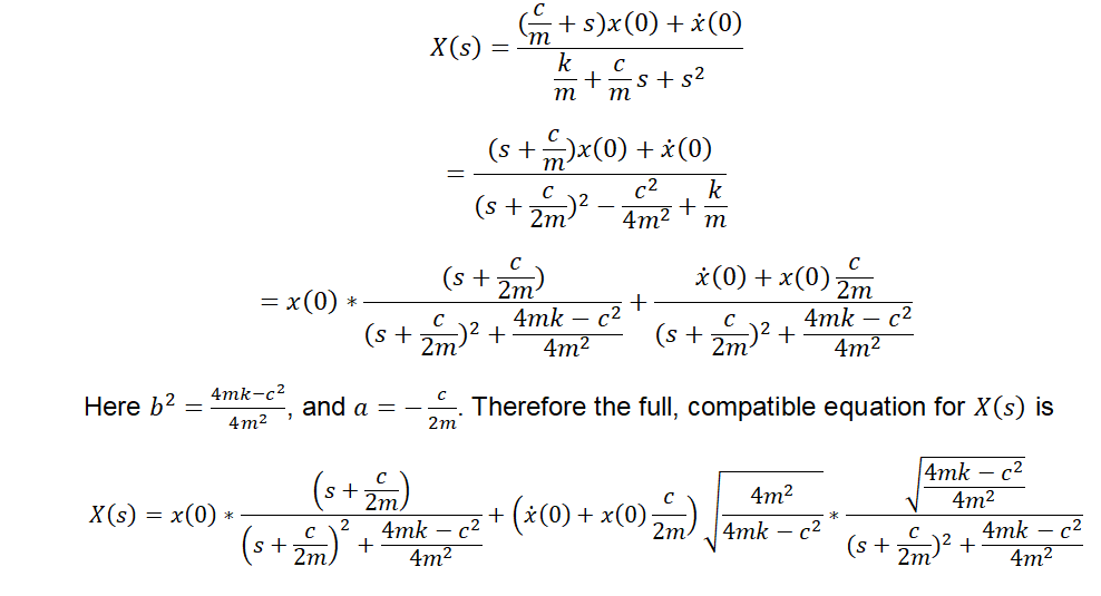
Rearrange to find X(s).

Rewrite it in a compatible way for reverse-Laplace transforming.

Therefore the formula for x(t) is

.

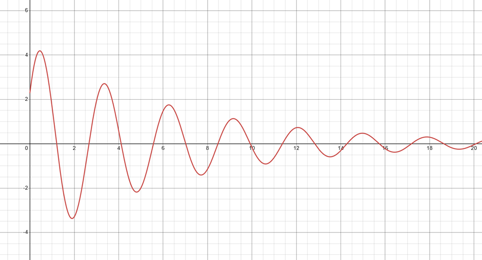
This is indeed the general solution for damped harmonic motion, where x(0) is the initial velocity of the spring k,  is the spring constant, C  is the damping constant, M  is the mass of the oscillating mass X(0) and  is the initial position. Plotting distance against time in Desmos also gives the expected graph.

Figure 2 -Graph here: https://www.desmos.com/calculator/ukieueypw8

Pros and cons

The benefit is clear: we can now have analytical, exact solutions to non-linear, “weird” differential equations (though both examples shown here were linear). This allows us to model more behaviours: for example, shockwaves can now be studied with the Burgers equation, allowing for advances in aerospace and fluid dynamics.

The benefit of a reverse-Laplace transform from a computer is less clear-cut, as iteration is less complicated and still provides. However, many conventional frameworks such as Dormand-Prince or RK4 require a first-order differential equation, while a Laplace transform can handle possibly infinitely many orders. Apart from this, the Laplace transform does not run into inaccuracies from making a time-step too large the same way iteration does. However, the Laplace transform is kind of hard to do if one cannot solve a complex integral, and calculating it with a computer can be a pain.

Conclusion

As such, the Laplace transform is a great tool to add to your mathematical arsenal; the above highlights how to do this. I encourage you to Laplace transform more differential equations in your spare time to practice this.

where  is the complex Laplace variable and  is the function you want to transform.

Don’t worry if you have never seen this before: this part is often done with a computer anyway. In essence though, the transform “translates” the function of  into a function of the Laplace variable, .